MATH/CS 5486 - NONLINEAR INVERSE PROBLEMS
In inverse problems, we recover an image of an unknown quantity of interest inside a given medium, such as electrical conductivity in human tissue, using a mathematical model that relates the image of the unknown quantity to the measured data (the forward model). Given the ubiquitous nature of inverse problems in fields such as geophysics, medical imaging, hydrology, and nondestructive evaluation, the need for innovative, efficient, and accurate algorithms for such problems is as great as ever.
Inverse problems combine a mathematical model of a physical process, governed by one or more unknown scalar fields, with (noisy) observations of its response to various stimuli to recover estimates of the scalar fields. The scalar fields, often referred to as an images, represent unknown quantities of interest: in medical imaging, an anomalous region of electrical conductivity in human tissue indicates possible tumor sites; in hydrology, an anomalous region of electrical conductivity underground indicates a possible contaminant plume.
|
|
|||
|
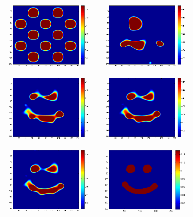
Example of Diffuse Optical Tomography (DOT) for image reconstruction using synthetic (computer generated) data. There are 32 sources at the top and 32 detectors at the bottom. The movie shows the initial approximation and first few approximate solutions for a second and then shows the steps of the reconstruction in a movie. |
This class introduces techniques for discretization, numerical linear algebra, in particular approximate solution techniques and model reduction, nonlinear optimization, and regularization to derive efficient methods for nonlinear inverse problems. Regularization refers to techniques that constrain approximate solutions or penalize undesirable features of approximate solutions (such as large oscillatory components) to define a well-posed reconstruction/optimization problem. In general, inverse problems are ill-posed, that is, the (exact) solution does not exist, is not unique, or does not depend continuously on the data (measurements); therefore, regularization is required to obtain meaningful solutions.
Instructor: Eric de Sturler
Prerequisites: As all relevant topics will be introduced in this course, but at a relatively fast pace, prerequisites are a reasonable background in numerical analysis and some programming experience in Matlab ®. This course can be taken independently from MATH/CS 5485, although taking MATH 5485 will help with parts of this course.
Overview: The first part of the course deals with linear inverse problems and is based on the book Discrete Inverse Problems by P.C. Hansen (published by SIAM). This part introduces the students to the basic features of inverse problems. The second part of the course deals with nonlinear inverse problems, especially those based on parameterized partial differential equations (PDEs), and will be based on lectures notes and slides prepared for this class and possibly some review papers.
Textbooks:
Lecture Notes:
The lecture notes will cover significant additional material (in particular for the 2nd
part of the course)
This material is based upon work supported by the National Science Foundation under Grant No. DMS-1217156, DMS-1217161, DMR-0325939, and DMS-0342559. Any opinions, findings, and conclusions or recommendations expressed in this material are those of the author(s) and do not necessarily reflect the views of the National Science Foundation.
